normalized cuts (graph-based)

• nodes = pixels
• edges = between pairsof pixels
  • affinity weight, measuring similarity, for each edge
  • similarity is inversely proportional to difference

goal

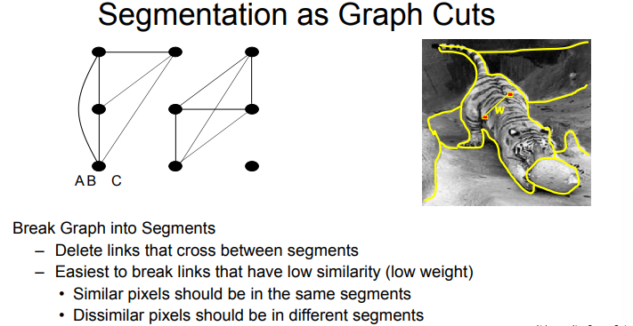
• cut graph into segments where
  • pixels in segments are highly similar
  • pixels across segments are dissimilar

1. construct graph - what edges?
   1. fully connected - all pairwise sims, but infeasible
   2. grid-based (neighboring pixels) -
      1. more efficient than fully connected graph
      2. only gets local interactions
   3. local neighborhood
      1. reasonably fast, graph still sparse
      2. good tradeoff
2. define similarity
   1. gaussian similarity
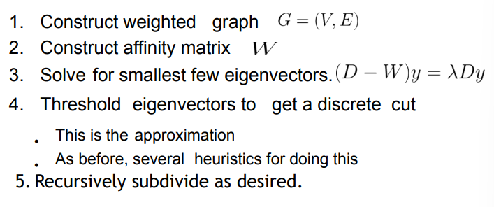
3. solve for e-vecs, eigenvectors+values
   1. formulate as graph laplacian problem
   2. eigenvectors give cluster assignments

segmentation as graph cuts

image as graph

• Every pixel is connected to its 8 neighboring pixels
• The edges between neighbors have weights that are determined by the distance between them.
• Edge weights between pixels are determined using dist(x, x’) distance in feature space.
  • where x and x’ are two neighboring pixel

segmentation as graph-cut

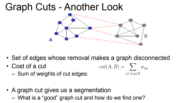
• S is segmentation of G where we keep all vertices but select subset of edges
• S divides G such that G’ contains distinct clusters

alternative

clustering via eigenvalue

1. Construct affinity matrix W
2. Compute eigenvalues and vectors of W
3. Until done
4. Take eigenvector of largest unprocessed eigenvalue
5. Zero all components of elements that have already been clustered
6. Threshold remaining components to determine cluster membership Note: This is an example of a spectral clustering algorithm

min cut

• smallest num of elements (unweighted) or smallest sum of weights (weighted) drawback
• weight of cut proportional to num edges
• biased towards cutting small, isolated components

better: normalize cuts

• avoid bias towards small clusters
• balances within-cluster sim and between-cluster dissim
• normalize segment size to fix min cut’s bias

pros

• elegant
• flexible to choice of affinity matrix

cons

• computationally heavy w many cuts
• bias towards balanced partitions
• constrained by affinity matrix model